From synthetic geometry to dynamic geometry and back: the case of circular inversion

by Giulia Signorini, Michele Tocchet, both from “Liceo Filippo Buonarroti” in Pisa, and Anna Baccaglini-Frank², University of Pisa.¹

Euclid’s V Postulate has always appeared less evident than the other axioms (maybe even to Euclid himself) and over the centuries it gave rise to many discussions, culminating with the advent of the so-called non-Euclidean geometries, that are based on its negations. For example, we can assume that given a point and a line on the plane there does not exist any line through the point and parallel to the given one, or we can assume that there exist infinitely many parallel lines to the given one through the point.

In 1871 Felix Klein published two papers [2, 3], called On the so-called non-Euclidean geometry, in which he proposed to call the first type of geometry “elliptic geometry” (from the Greek ellipsis, that means omission) and the second type “hyperbolic geometry” (form the Greek hyperbola, that means excessive).

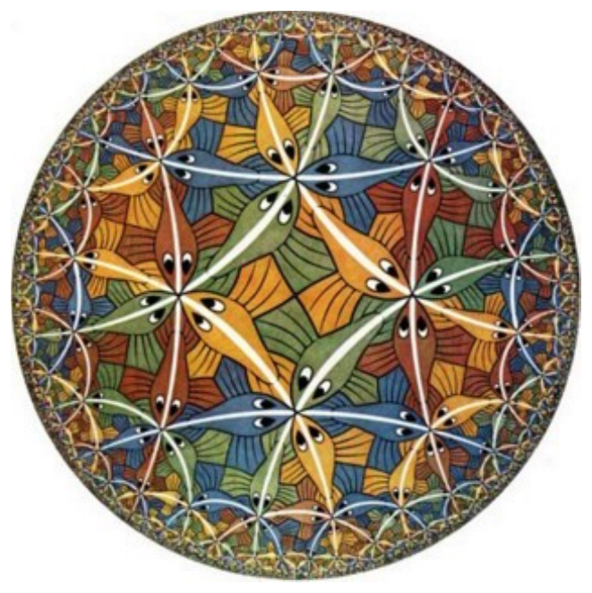
Figure 1. Hyperbolic tessellation of Poincaré’s disk by M.C. Escher (Circle Limit III by M. C. Escher, 1959).

A good model for elliptic geometry is the sphere, while a model for hyperbolic geometry, for example, is Poincaré’s disk (there are other models, including one proposed by Klein himself, but these are usually considered to be less intuitive), a disk with a different metric from the Euclidean metric in which the points on the boarder are “points at infinity” and the objects become smaller and smaller as they approach the boarder of the disk.

While thinking about geometry on a sphere is relatively easy, since we are lucky enough to be living on one, imagining Poincaré’s disk is more difficult and intriguing, indeed it has even inspired artists such as M. C. Escher (to see other beautiful artwork by Escher we recommend visiting the official website of the M.C. Escher Foundation at www.mcescher.com). To gain an elementary intuition about the Poincaré disk frequently a particular transformation of the plane is introduced: circle inversion.

Circle inversion provides an interesting example of geometric transformation that, unlike the affinities and isometries studied in high school, usually does not transform lines into lines (but into circles) and that can be presented in an elementary way since its properties can be explored with dynamic geometry software and easily proved in synthetic geometry. Indeed, some high school textbooks introduce circle inversion as an interesting topic of Euclidean geometry that can also be explored through dynamic geometry software³.

Let us take a look at some of its properties, starting from its definition and construction.

1. Circle inversion

Let us start with the definition of circle inversion (or inversion) of a point P.

Given a circle $C$ with center $O$ and radius $r$ and a point $P$ different from $O$ , we define the inverse of $P$ with respect to $C$ a point $P'$ on the ray $OP$ such that⁴ $OP \cdot OP' = r^2$ .

As we mentioned above, in this context it can be interesting – and sometimes surprising – to explore the characteristics of the transformation we defined, using a software for dynamic geometry. Many such environments contain a command “circle inversion” (the figures in this vignette are sketched using the free software GeoGebra).

Figure 2. Inverse of a point $P$ that is internal or external to the reference circle.

Interacting with the software, or even just thinking about the definition and recognizing its symmetry, one can deduce that it is an involution of the plane⁵ and that the image of a point inside the circle will be farther from $C$ the closer it is to its center and vice versa, and the points on the circle are fixed points of the transformation.

Another useful definition is that of power of a point P.

The power of $P$ with respect to the circle $C$ is written as $\prod_C P$ and defined as the product $PA \cdot PB$ , where $A$ and $B$ are the points of intersection of any line through P with the circle $C$ .

Since the lines involved in this definition are infinitely many, we need to check that $\prod_C P$ is indeed well-defined, that is, that it does not depend on the line chosen.

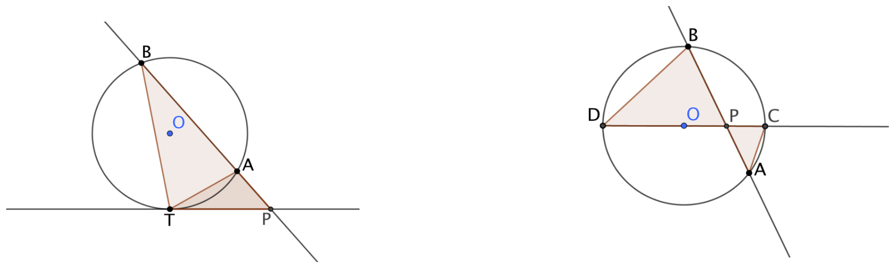
Figure 3. Secant-tangent theorem and chord theorem.

This check follows immediately from the chord theorem (in the case in which $P$ is inside the circle) and from the secant-tangent theorem (in the case in which $P$ is outside the circle), both usually introduced in Euclidean geometry at the high school level.

We note that, since the quantity $\prod_C P = PA \cdot PB$ is invariant no matter which line through $P$ is chosen, it is always possible to choose the line through the center $O$ of the circle, that is, the line that contains a diameter of $C$ . Therefore, we can show that

$\prod_C P = |OP^2 - r^2|.$

Since this will be very useful later on, we will refer to this equality as propriety zero of the power of a point $P$ with respect to $C$ .

2. First properties

A first property of inversion, that is a bit less evident, is the following. Since it does not immediately follow from the definition, we will call it Theorem 1.

If $P'$ is the inverse of $P$ with respect to $C$ , for every point $Q$ of the circle $C$ the ratio between the segments $PQ$ and $P'Q$ remains constant.

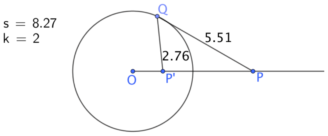
In fact, there is no apparent reason why this theorem should be true: the invariance of the ratio no matter how we choose $Q$ seems to be something “magical”. The surprise effect can be amplified (and therefore used didactically as a stimulus for searching for a proof) by trying it in dynamic geometry, for example dragging $Q$ along the circle and checking explicitly that the ratio between the lengths of $PQ$ and $P'Q$ remains constant (in Figure 3 we chose to show both the sum $s$ between the lengths of the two segments and their ratio $k$ , to show even more evidently that the first changes while $Q$ moves along the circle, while the second remains constant).

Figure 4. Exploration and testing in dynamic geometry.

We now prove Theorem 1.

An analytical proof for Theorem 1 is possible using the analytical expression for inversion, but we prefer to work synthetically, as shown below.

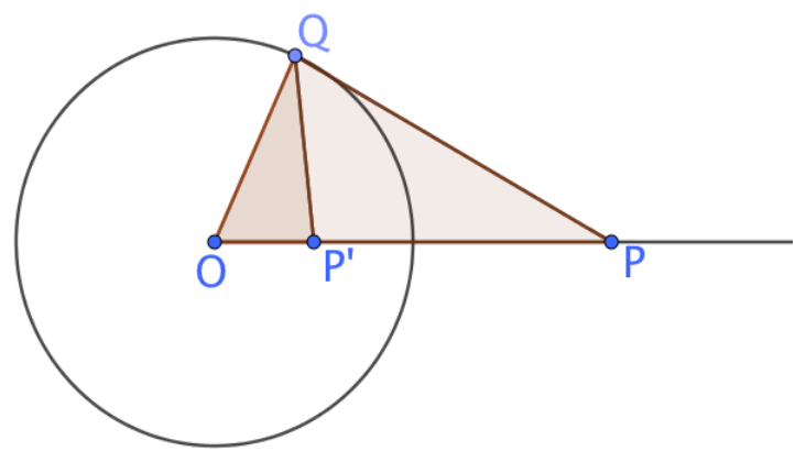
Since point $P'$ is the inverse of $P$ , we know that $OP \cdot OP' = r^2$ (where $r$ is the radius of the circle). This is equivalent to saying that $OP'/r = r/OP$ and therefore, since point $Q$ belongs to circle $C$ , that $OP'/OQ = OQ/OP$ (we remind the reader that we assumed that $P$ is different from $O$ , so dividing by $OP$ is never a problem).

Therefore we consider the two triangles $QOP$ and $QOP'$ : the preceding equality guarantees that their sides are proportional and the angle $\angle QOP'$ is common to both triangles, therefore the triangles $QOP$ and $QOP'$ are similar.

So we can write the proportion relating the third sides of both triangles, and get $QP'/QP = OP'/QO$ . From this equality, remembering that $P'$ is the inverse of $P$ and that therefore $OP' = r^2/OP$ and that $Q$ belongs to the circle $C$ so $OQ = r$ , we can conclude that $QP'/QP = r/OP$ .

Since the ratio $r/OP$ is determined only by the position of $P$ and it does not depend from our choice of $Q$ , we proved what we wanted.

Moreover, notice that this proof is the same whether $P$ is outside or inside the circle: the property in Theorem 1 is true in both cases.

This way we can see that together with the proof of Theorem 1 we also reached an expression for the constant as a function of the radius $r$ and of the point $P$ : $QP'/QP = r/OP$ .

3. From the properties to a new construction method

Until now we only used dynamic geometry to explore properties and check theorems (and also to make drawings that are more precise than those we could have drawn by hand with pencil and paper!). The potentials of dynamic geometry software, however, go well beyond these: we can make use of the many examples and counter-examples that we can generate by dragging the dynamic objects to make or refute conjectures. Circle inversion is a great context for doing this.

Let us consider a circle $C$ with center $O$ , point $P'$ is the inversive image of $P$ ; as in the definition of the power of a point with respect to $C$ , let us mark as $A$ and $B$ the two intersection points of any line through $P$ that intersects the circle. Then let us consider point $B'$ the image of $B$ through line symmetry over $OP$ . Notice that since Theorem 1 is true for any point of $C$ , it must also be true for $A$ , for $B$ and for $B'$ .

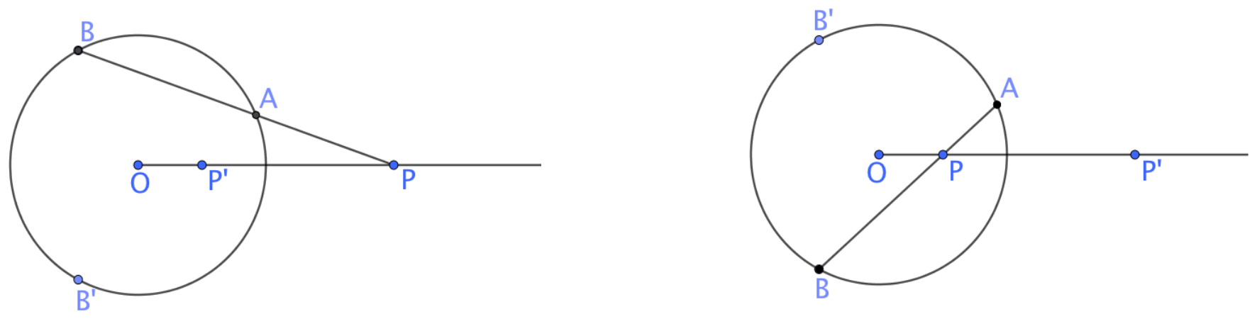Figure 6. Construction of points $A$ , $B$ and $B'$ on the circle.

In the figures above we decided to apply line symmetry to one of the points of intersection between the line and the circle, and specifically to the point that had a greater distance from $P$ , but we could have chosen either point of intersection to reflect (indeed the choice of which point to call $A$ and which to call $B$ is completely arbitrary).

Moreover, for sake of brevity, we will only refer to the case in which $P$ is outside the circle $C$ , but we are sure that the curious reader can treat the case in which $P$ is inside (only small variations to our work below need to be made).

If now we try to continuously vary the figure, dragging point $B$ along the circle, we can notice that points $A$ , $P'$ and $B'$ seem to always stay aligned, even when $B$ and $B'$ switch places on $C$ .

So, interacting with the construction we figured out something new and “magical”: it looks like we have found a new property of $P'$ the inverse of $P$ with respect to $C$ .

But can we trust our perception? Will the three points actually always be aligned? To be more sure we can always ask the software to measure the angles $\angle B'P'O$ and $\angle AP'P$ and visually verify that their measures (up to two decimals of a degree) are always the same no matter where $B$ moves along the circle.

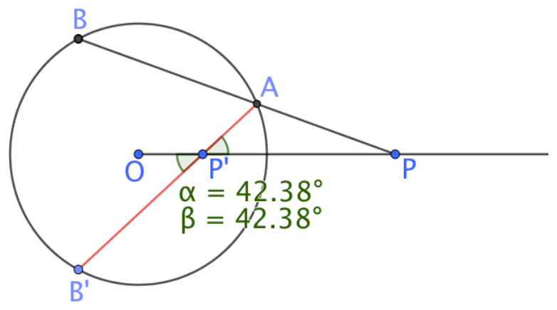
Figure 7. Check the alignment of the points through angle measures.

We could then ask ourselves if it is $P'$ that is “special”, or if this new property uniquely identifies the inverse of a point with respect to circle inversion.

To verify this conjecture we consider any point $K$ on segment $OP$ and we construct the segments $B'K$ and $AK$ . Thanks to dynamic geometry, varying the position of the points continuously, we can generate infinitely any examples and counter-examples, and we can verify visually that dragging $K$ along $OP$ and $B$ along $C$ , points $A$ , $K$ and $B'$ seem to line up only when $K$ coincides with $P'$ , and in this case the points seem to stay aligned no matter how we move $B$ .

Figure 8. Check of the characteristic property of $P'$ .

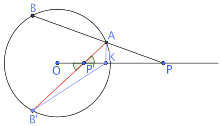This second exploration should have finally convinced us that our conjecture can be proved: it seems that we have found a new invariant through which we can define the inverse of a point on the plane!

So now we are ready to state and prove our discovery, which we will call Theorem 2.

Given a circle $C$ with center $O$ and radius $r$ and a point $P$ different from $O$ , and let $A$ and $B$ be the points of intersection of any line through $P$ with $C$ , $B'$ the symmetric image of $B$ across the line $OP$ and $P'$ a point of the ray $OP$ . Then the points $A$ , $P'$ and $B'$ are aligned if and only if $P'$ is the inverse of $P$ with respect to the circle $C$ .

If to generate our conjecture we could make use of dynamic geometry, to finally prove Theorem 2 we have to use Euclidean Geometry: if in fact our conjecture holds, we should be able to prove it through a chain of implications using other known theorems!

Let us start by proving that if $P'$ is the inverse of $P$ with respect to the circle $C$ , then points $A$ , $P'$ and $B'$ lie on a line.

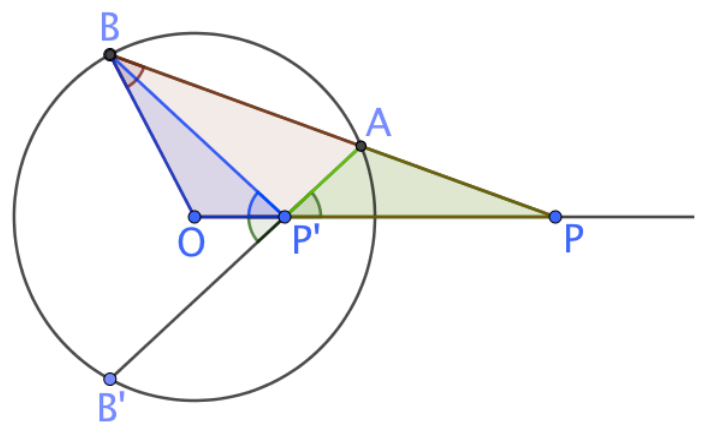
Figure 9. Proof of the first implication in Theorem 2.

Let us consider the triangles $OBP$ and $AP'P$ . Since $P'$ is the inverse of $P$ with respect to the circle $C$ we know that $OP \cdot OP' = r^2$ . We can change signs and add $OP^2$ to both sides of the equality, and we get $OP^2 - OP \cdot OP' = OP^2 - r^2$ . From the left side we can factor out $OP$ and substitute the difference $(OP - OP')$ with $P'P$ , while – recalling property zero of the power of a point – on the right hand side we can recognize $\prod_C P$ . Therefore by using the definition we can transform it into the product $PA \cdot PB$ , and get $OP \cdot P'P = PA \cdot PB$ , which is the equality between the ratios $OP/PB = PA/P'P$ . Since the triangles have angle $\angle BPO$ in common, we can conclude that the triangles $OBP$ and $AP'P$ are similar. So the angles $\angle AP'P$ and $\angle OBP$ are congruent.

On the other hand, looking at the proof of Theorem 1 applied to point $B$ we also find that the triangles $OBP$ and $OBP'$ are similar, from which we deduce that the angles $\angle OBP$ and $\angle OP'B$ are congruent.

Therefore it is enough to observe that the angles $\angle OP'B$ and $\angle OP'B'$ are congruent by construction to conclude that $\angle AP'P = \angle OP'B'$ and so the three points $A$ , $P'$ and $B'$ must lie on a line.

Next let us prove that also the vice versa is true, that is, if points $A$ , $P'$ and $B'$ lie on a line, then $P'$ is the inverse of $P$ with respect to $C$ .

Figure 10. Proof of the second implication of Theorem 2.

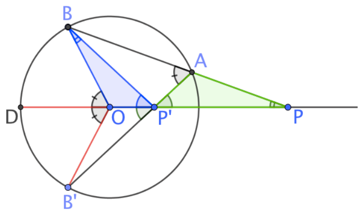
Let us consider the triangles $OBP'$ and $APP'$ . We call $D$ the intersection between line $OP'$ and $C$ on the opposite side of $P$ ; then by construction $\angle DOB = \angle DOB' = \frac{1}{2}\angle BOB'$ and they are all congruent to the angle $\angle BAB'$ , because $\angle BAB'$ and $\angle BOB'$ are respectively an inscribed angle and a central angle insisting on the same arc with endpoints $B$ and $B'$ . Moreover, since our hypothesis is that $A$ , $P'$ and $B'$ lie on the same line, the angle $\angle BAB'$ coincides with the angle $\angle BAP'$ . Therefore, using the exterior angle theorem, we get $\angle P'BO = \angle DOB - \angle OP'B = \angle BAP' - \angle AP'P = \angle APP'$ . This result, together with the alignment hypothesis, guarantees that $\angle AP'P = \angle OP'B'$ and since, by construction, $\angle OP'B' = \angle OP'B$ , it allows us to conclude that the triangles $OBP'$ and $APP'$ have a pair of congruent angles and therefore they are similar.

From this similarity we get that the equality $OP'/BP' = AP'/PP'$ holds. Since by construction $BP'$ is equal to $B'P'$ we can write $OP' \cdot PP' = AP' \cdot B'P'$ , that is $OP' \cdot PP' = \prod_C P'$ . Property zero of the power of a point allows us to transform this equality into $OP' \cdot PP' = r^2 - OP'^2$ , from which, substituting $PP'$ with $OP - OP'$ , we obtain $OP' \cdot (OP - OP') = r^2 - OP'^2$ .

Expanding the product on the left hand side, our equality becomes $OP' \cdot OP - OP'^2 = r^2 - OP'^2$ , which is $OP' \cdot OP = r^2$ . This is exactly what we wanted to prove.

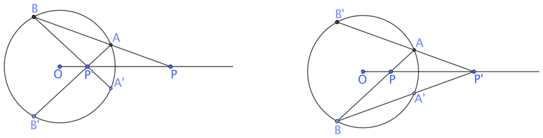
Interestingly, the invariant that we proved with Theorem 2, not only gives us a new property of circle inversion, but it also gives us an alternative method for constructing the inverse of $P$ with respect to circle $C$ .

This is the new construction protocol.

Given a circle $C$ with center $O$ and radius $r$ and a point $P$ different from $O$ :

draw any secant⁶ to $C$ through $P$ ;
construct the symmetric of one of the two intersection points with respect to the line $OP$ ;
draw the segment that connects this point with the other point of intersection;
call $P'$ the point of intersection between this segment and the line $OP$ ;

Theorem 2 guarantees that $P'$ is the inverse of $P$ with respect to $C$ .

Figure 11. Construction of the inverse of P in the cases of P being outside or inside the inversion circle.

4. A glance at history

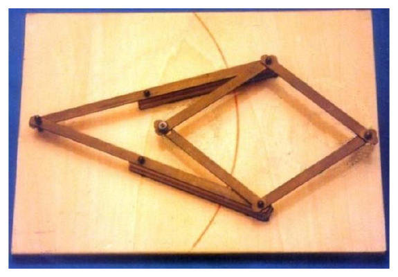
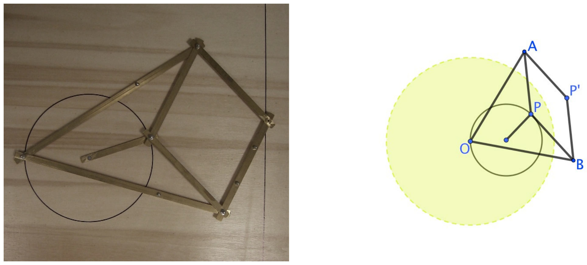
Figure 12. Physical recontruction of Peaucellier’s inversor.

Historically, the problem of constructing the inverse of a point $P$ was solves in 1864 by A. Peaucellier with the linkage in the figure below, known as the Peaucellier’s inversor [5].

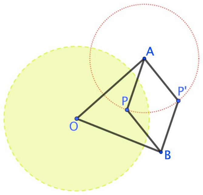
The mechanism is made up of two bars of equal length linked to the plane at a fixed point $O$ . Four other bars are linked to the endpoints of these bars; these four bars are congruent but shorter than the first two, and they come together at points $P$ and $P'$ making a deformable rhombus. Moving $P$ , the point $P'$ traces its inverse.

This mechanism can be constructed with dynamic geometry software, using six segments that come together at points $O, A, P, B, P'$ .

The circle of inversion is not part of the linkage, but we decided to represent it to help show the properties of circle inversion.

Using the secants theorem with the lines $OP$ and $OA$ , secant to the circle with center at $A$ and radius $AP$ , we can prove that $P'$ is in fact the inverse of $P$ with respect to the circle with center $O$ and radius $\sqrt{OA^2 - AP^2}$ .

Figure 13. Reconstruction with dynamic geometry software of Peaucellier’s inversor.

The importance of Peaucellier’s inversor is related to the problem of constructing a system to convert exact straight-line motion to circular motion, that at the end of the 18th Century was afflicting engineers who were looking for an effective way of transforming the straight-line up and down motion of a piston in a cylinder into the circular motion of the wheels of a steam engine.

Referring to Euclidean geometry we can easily prove that circle inversion transforms circles through the center of inversion into lines (and vice versa), so linking point $P$ to a circle through $O$ with a seventh bar forces $P'$ to move along a line. So Peaucellier’s mechanism provides an exact solution to the problem.

Figures 14 e 15. Physical and digital reconstruction of Peaucellier’s mechanism.

References

[1] A. Baccaglini-Frank, How I Stumbled Upon a New (to me) Construction of the Inverse of a Point. Digit Exp Math Educ 2, 278–287 (2016). https://doi.org/10.1007/s40751-016-0023-7

[2] F. Klein, Über die sogenannte Nicht-Euklidische Geometrie. Mathematische Annalen IV, 573-625 (1871).

[3] F. Klein, Über die sogenannte Nicht-Euklidische Geometrie (Zweiter Aufsatz) Mathematische Annalen VI, 112-145 (1873).

[4] A. Cuoco & CME Authors, The CME Project Geometry, Pearson (2008). http://cmeproject.edc.org

[5] E. W. Weisstein, Peaucellier Inversor. MathWorld–A Wolfram Web Resource. https://mathworld.wolfram.com/PeaucellierInversor.html

Figure 1 is a reproduction of Circle Limit III by M. C. Escher. Wood engraving, 1959.

The pictures of the physical reproductions of Peaucellier’s inversor (Figures 12 and 14) are reproduced from: http://www.macchinematematiche.org

Notes

Inspired by the snapshot: “How I Stumbled Upon a New (to me) Construction of the Inverse of a Point” [1].
University of Pisa (Italy). Contact per Email: anna.baccaglinifrank@unipi.it
A very good example of how this can be done is in Chapter 5 of “Geometry” in the CME Project high school textbooks [4].
In this vignette the notation $AB$ represents the length of the segment with endpoints $A$ and $B$ .
This is possible as long as we introduce a point at infinity and extend the inversion, by definition, to interchange the center O and this point at infinity.
Using dynamic geometry software it is easy to check that if $P$ is outside the circle, the method works analogously, even choosing one of the lines through $P$ that are tangent to the circle.

PDF

From synthetic geometry to dynamic geometry and back: the case of circular inversion

Related

Leave a ReplyCancel Reply

Share this:

Related

Leave a ReplyCancel Reply