Originating author is Nitsa Movshovitz-Hadar.
Prolog

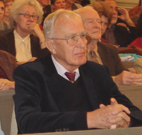
This article is an English translation with emendations of a Hebrew paper written in 2014 about two years after the untimely passing of the illustrious lecturer and group theory expert, Professor David Chillag. It is dedicated to commemorating him. He entrusted me with the transparencies that accompanied his lecture on the enormous theorem presented in 2011 at the Technion Mathematical Club, hoping to produce a paper for teachers and teachers’ teachers on the subject. Unfortunately, we did not manage to do it together.
I thank those of our mutual colleagues who helped me with this$^1$, and at the same time, of course, I take full responsibility for things that are not entirely clear or even incorrect.
Nitsa Movshovitz-Hadar
Introduction – What is this article all about?
The definition of a group in mathematics is an abstraction of the set of integers with the familiar operation of addition. A group is a set (such as the integers) with a binary operation which enables combining any two elements in the set and get as a result one element in the set (such as the sum of two integers), that has a few simple properties such as the existence of a unique “neutral element” (zero in the case of the integers). There is a large wealth of mathematical groups, differing from one another in composition and size. Some of them consist of a finite set (such as the set $\{0,1,2,3,4,5,6,7,8,9,10,11\}$), others consist of an infinite one (such as the integers). The binary operations vary as well (think, for example, about addition-modulo-$12$ defined on the finite set mentioned earlier$^2$, or about addition defined on the integers). The wealth of mathematical groups is so large that there is no chance of classifying even the finite ones of them. Fortunately, there is a special family of finite groups called simple finite groups, which can be classified. It turns out that this special family of finite groups is of great importance because, in some sense, all finite groups can be built from simple finite groups in a way that is somewhat analogous to the fact that all the positive integers can be built from the prime ones. The “enormous theorem,” the subject of this article, gives a complete classification of the simple finite groups. In this way, it provides tools for analyzing the structure and features of all finite groups. The theorem received its “enormous” nickname for some very good reason, to be explained below.
Let us meet the people behind the scene.
The people behind the scene

On November 2, 2011, at a ceremony in Stockholm, Sweden, the Rolf Schock Prize in mathematics$^3$ was awarded to Professor Michael Aschbacher of Caltech – the California Institute of Technology, “… for his fundamental contributions to one of the largest mathematical projects ever, the classification of finite simple groups…”$^4$
The program for the classification of simple finite groups project, undoubtedly one of the most ambitious projects in pure mathematics that have ever been conceived, was outlined in 1972 by Prof. Daniel Gorenstein, a mathematician at Rutgers University, USA. His idea was to tie together various disparate strands of mathematical studies published from the mid-20th century on, rooted in the work that began as early as the 19th century, and turn them into a concerted classification program.
Nine years later, in 1981, Robert Greiss constructed “The Monster Group”, which is a simple finite group with as many as $8\cdot 10^{53}$ elements. This discovery led Gorenstein to his proclamation made in 1983: “In February 1981, the classification of simple finite groups was completed”.

The announcement of the completion of the classification, which is nowadays considered a landmark in contemporary mathematics, was met with skepticism from the outset and did not receive any special public attention. Why? – Because its proof was controversial. It spanned more than 10,000 pages and was spread across some 500 articles published in various journals and written by over 100 different authors from all over the world. This was an unprecedented case in the history of mathematics. Some skeptics were right – indeed, the proof turned out to require corrections here and there, mostly done between 1995 and 2004.
Michael Aschbacher’s great contribution was the result of seven years of work, during which he and his colleague Stephen Smith published two additional voluminous books on solving the issue, until in 2004, Aschbacher wrote: “to my knowledge the main theorem [of our recent work] closes the last gap in the original proof, so (for the moment) the classification theorem can be regarded as a theorem.”
What exactly does the theorem state, and why does it require such a lengthy proof? What are “simple finite groups”? What does it mean to “classify” them? And what is the significance of such classification? The rest of this article is devoted to clarifying these questions. Let us start from the basic one –
What are “simple finite groups”?
This question, in itself, has three parts. Firstly, we need to understand what a group is, then what is a finite one, and lastly, what is a simple finite group.
A group is a non-empty set $G$ with a binary operation $*$ that is well defined$^5$ on any pair of elements in $G$ satisfying the following four requirements:
- Closure: $a*b \in G$ for all $a,b \in G$, namelythe result of the operation is an element in $G$ for any two elements $a$ and $b$ in$ G$.
- Associativity: $(a*b)*c=a*(b*c)$ for all $a,b,c \in G$, namely, the result of combining any three elements $a,b,c$ in $G$ is the same whether we initially combine $a$ and $b$ then combine the result with $c$, or we start by combining $b$ and $c$ then combine $a$ with the result.
- Existence of a neutral element: There exists in $G$ an element $e$ that satisfies $a*e=e*a=a$ for any element $a$ in $G$.
- Existence of a reciprocal element to each element: For every element a in $G$, there is a reciprocal element $a^{-1}$ in $G$, which satisfies $a*a^{-1}=a^{-1}*a=e$.
Note: The definition of a group does not require the commutativity of the operation. Namely, it is not necessarily true that for any two elements $a,b$ in $G$, $a*b=b*a$ (some pairs of elements may commute, but at least one pair doesn’t). Everything from here on holds for any group, no matter if the operation is commutative or not.
The number of elements in the set $G$ can be finite or infinite. For example, the infinite set of integers with the operation of addition is an infinite group (with zero as the neutral element). So is the infinite set of rational numbers that differ from zero, with the operation of multiplication (here $1$ in the neutral element).
A finite group is a group that consists of a finite number of elements in G. The “clock group” is an example of a finite group that consists of the finite set $\{1,2,3,4,5,6,7,8,9,10,11,12\}$ with the addition-modulo-$12$ operation (where $12$ is the neutral element). Another example is the set of symmetries of the square, namely the rigid transformations that place a square onto itself. There are $|G|$ commonly designates the number of elements in a finite group $G$ eight such transformations: four turns around the intersection of the two diagonals (at $90$ degrees designated $R_{90}$, $180$ degrees – $R_{180}$, $270$ degrees – $R_{270}$, and $360$ degrees – $R_{360}$) and four reflections – in each of the two diagonals (designated $D_1$, $D_2$), and in each of the two middle lines (designated $H$ for the horizontal one, and $V$ for the vertical one). The binary operation is the successive performance of any two of these eight transformations. The Cayley-table of this operation shows the results this operation yields for any pair of these eight transformations. Each of the results is one of the eight transformations. Hence the set is closed under the operation of successive performance, which is sometimes called “followed by.”

The reader is invited to double-check the results by experimenting: take a square-paper, mark its vertices $A, B, C, D$, (on both sides of the square paper) and perform any two of the eight transformations one after the other; note the end position of the four vertices; then find the single transformation that yields the same end position. Verify your findings by the result shown in the Cayley-table.
As can also be seen from the table above, the neutral element is the rotation by $360^\circ$ and each transformation has a reciprocal one that combined together yield the neutral transformation. By the way, this group is non-commutative, which as well can be seen from the table by looking, for example, at the two different results of performing a horizontal flip followed by a $90$-degree rotation as compared to a $90$-degree rotation followed by a horizontal flip.$^6$
Note that $|G|$ commonly designates the number of elements in a finite group G, and usually, it is referred to as the order of the group.$^7$ By the way, as early as in the year 1872, the notable German mathematician and mathematics educator Felix Klein (1849- 1925) published the Erlangen Program in which he proposed to sort and explore the various geometries by their symmetry groups.
As mentioned earlier, this article focuses on simple finite groups. Before we turn to the definition of a simple finite group, we should discuss the notion of a subgroup. A subset $S$ of a finite group $G$ is a subgroup if and only if it is closed under the operation of the group. For example, the four turns in the group of eight symmetries of the square form a subgroup of order $4$ (The reader is welcome to check it using the above Cayley-table). A subgroup of order $2$ of the same group is formed by any one of the four reflections and the identity transformation (which must be included in any subgroup). Clearly, the orders of these subgroups divide the order of the group. This is not accidental. It is the general case, as proved by Lagrange (1736-1813), that the order of any subgroup of a finite group divides the order of the group.$^8$ It is worth noting that every group has two “trivial subgroups”: the subgroup that contains the neutral element only, and the whole group itself. (This is somewhat similar to the well-known fact that any positive integer $n$ has divisors, of which two are trivial: $1$ and $n$ itself.) There is a special type of subgroups called normal subgroups, which is the key to understanding the notion of a simple finite group. A subgroup $H$ of $G$ is called normal if and only if for every element $h$ in $H$ and every element $g$ in $G$ the element $g*h*g^{-1}$ is also in $H$. It is quite easy to see that the two trivial subgroups of any group are normal (the reader can clarify this point by going back to the definition of the two trivial subgroups and examine their fulfillment of the condition for being normal.) Therefore every group has at least two normal subgroups. It is also easy to see that in a commutative group, every subgroup is normal$^9$. Now we are ready for the definition:
A finite group $G$ is called simple if and only if it does not have any normal subgroup other than the two trivial ones. (Note the similarity again to the definition of a prime number as a positive integer that does not have any divisors other than the two trivial ones.)
It turns out that the simple finite groups are the building blocks of all the finite groups, in a comparable way to that of the positive prime numbers being the (multiplicative) building blocks of the natural numbers. Comparable – however, a bit more complicated. Let us see how –
For each group $G$ and any of its normal subgroups $H$, a new group can be defined – the so-called quotient group $G/H$.$^{10}$ The structure of the subgroup $H$ and the structure of the quotient group $G/H$ shed light on the structure of $G$. This is due to a basic theorem in group theory, proved in the late 19th century, called the Jordan-Hölder theorem, which is a far-reaching generalization of the fundamental theorem of arithmetic (the unique factorization of the positive integers into primes). It states that every finite group can be decomposed into an increasing series of subgroups $H(1), H(2),…, H(n)$ such that $H(i)$ is a normal subgroup of $H(i+1)$, and the quotient groups $K(i) = H(i+1)/H(i)$ are all simple groups.
Moreover, the decomposition series $\{K(i)\}$ is unique, namely if there is another series of quotient groups $\{L(i)\}$ obtained in the same way and all of them are simple, then the two series are equivalent, in other words, they are of the same length and each quotient group in one series is isomorphic$^{11}$ to one and only one of the quotient groups in the other series. That is to say, the two series of quotient groups $\{K(i)\}$ and $\{L(i)\}$ are not different from one another except possibly for the order of their elements. The Jordan- Hölder theorem indicates a close relationship between finite groups and simple finite groups.$^{12}$
The eagerness of mathematicians specializing in group theory to map and classify the simple finite groups stemmed from their curiosity to find out more about the properties of the entire family of finite groups. This is analogous to the curiosity of number theorists about the natural prime numbers, which stemmed from their wish to find out more about the entire family of the positive integers.
What does it mean to “classify” the simple finite groups?
The classification of triangles in the Euclidean plane, which is based upon the notion of congruence, is a simple example for the treatment of the classification of a family of mathematical objects. Two triangles that can be obtained from one another by an isometric transformation (a distance preserving transformation) are not considered distinct objects for the sake of giving a detailed list exhausting all the various objects which satisfy the definition of a triangle and enabling the analysis of their properties. Another familiar example is the classification theorem of the Platonic solids, which states that there are exactly five types of objects satisfying the definition of polyhedron made of regular congruent planar polygonal faces with the same number of faces meeting at each vertex: Tetrahedrons, Cubes (or hexahedrons), Octahedrons, Dodecahedrons, and Icosahedron. Analogously, the classification theorem of the family of simple finite groups, the proof of which has been completed in the first decade of this century, presents a detailed and exhaustive list of all and only distinct abstract objects that satisfy the definition of a simple finite group, not distinguishing between two isomorphic ones.
Here are a few examples in this list.
Consider the finite group $Z_p =\{0,1, 2,…, p − 1\}$ with the addition-modulo-$p$ operation (e.g. the “7-days” group). Any other finite group $G$ consisting of $p$ elements where $p$ is a positive prime, $|G|=p$, is isomorphic to this group. Since $p$ is a prime number, it has no non-trivial divisors. Therefore, by Lagrange’s theorem, $Z_p$ has no non-trivial subgroups. In particular, it does not have any non-trivial normal subgroups. Hence it is a simple group. As there are infinitely many positive primes, this is an infinite family of such simple finite groups (a countably infinite one). In the list of all the simple finite groups, this infinite family appears under the general representation using the parameter $p$. The groups in this family have a unique property. These are the only commutative simple finite groups.
Are there other infinite families that are not isomorphic to $Z_p$? – The answer is yes. Between the years 1800 and 1960, eighteen distinct (non-isomorphic) infinite families of simple finite groups were identified by various mathematicians, notably Galois, Jordan, Dickson, Chevalley, Tits, and Suzuki.
As of 1960, no other such infinite families were found. However, a few simple finite groups that do not belong to any of the $18$ infinite families were discovered. To illustrate it let us consider two $11\times 11$ square matrices:
$A= \left( \begin{array}{rrrrrrrrrrr}
0 & 1 & 0 & 0 & 0 & 0 & 0 & 0 & 0 & 0 & 0\\
0 & 0 & 1 & 0 & 0 & 0 & 0 & 0 & 0 & 0 & 0\\
0 & 0 & 0 & 1 & 0 & 0 & 0 & 0 & 0 & 0 & 0\\
0 & 0 & 0 & 0 & 1 & 0 & 0 & 0 & 0 & 0 & 0\\
0 & 0 & 0 & 0 & 0 & 1 & 0 & 0 & 0 & 0 & 0\\
0 & 0 & 0 & 0 & 0 & 0 & 1 & 0 & 0 & 0 & 0\\
0 & 0 & 0 & 0 & 0 & 0 & 0 & 1 & 0 & 0 & 0\\
0 & 0 & 0 & 0 & 0 & 0 & 0 & 0 & 1 & 0 & 0\\
0 & 0 & 0 & 0 & 0 & 0 & 0 & 0 & 0 & 1 & 0\\
0 & 0 & 0 & 0 & 0 & 0 & 0 & 0 & 0 & 0 & 1\\
1 & 0 & 0 & 0 & 0 & 0 & 0 & 0 & 0 & 0 & 0\\
\end{array}\right) $
$B=\left( \begin{array}{rrrrrrrrrrr}
1 & 0 & 0 & 0 & 0 & 0 & 0 & 0 & 0 & 0 & 0\\
0 & 1 & 0 & 0 & 0 & 0 & 0 & 0 & 0 & 0 & 0\\
0 & 0 & 0 & 0 & 0 & 0 & 1 & 0 & 0 & 0 & 0\\
0 & 0 & 0 & 0 & 0 & 0 & 0 & 0 & 0 & 1 & 0\\
0 & 0 & 0 & 0 & 0 & 1 & 0 & 0 & 0 & 0 & 0\\
0 & 0 & 0 & 1 & 0 & 0 & 0 & 0 & 0 & 0 & 0\\
0 & 0 & 0 & 0 & 0 & 0 & 0 & 0 & 0 & 0 & 1\\
0 & 0 & 1 & 0 & 0 & 0 & 0 & 0 & 0 & 0 & 0\\
0 & 0 & 0 & 0 & 0 & 0 & 0 & 0 & 1 & 0 & 0\\
0 & 0 & 0 & 0 & 1 & 0 & 0 & 0 & 0 & 0 & 0\\
0 & 0 & 0 & 0 & 0 & 0 & 0 & 1 & 0 & 0 & 0\\
\end{array}\right) $
In the middle of the 19th century, a French mathematician Émile Leonard Mathieu$^{13}$ (1835-1890) showed that performing all the possible multiplications of $A$ and $B$ with repetitions (e.g. $AB^3$ $A^7$ $BABA^8$ ) yields a set of $11\cdot 10\cdot 9 \cdot 8=7920$ matrices which forms a simple group under matrix multiplication (non-commutative, obviously)$^{14}$. When it became clear that this group is not isomorphic to any of the groups in any of the $18$ already known infinite families of simple finite groups, it was named after Mathieu, its discoverer $- M_{11}$ .

In a similar way, by 1873, Mathieu discovered additional four simple finite groups that can be represented as permutation groups on $11, 12, 22, 23, 24$ objects. They also were named after him: $M_{12},M_{22},M_{23},M_{24}$ respectively, and are referred to as sporadic, as they do not belong to any of the $18$ infinite families.
Almost 100 years passed since Mathieu’s discoveries with no progress. He passed away in 1890, and only in 1966, a new sporadic simple finite group was surprisingly discovered, by a Croatian mathematician Zvonimir Janko (born 1932)$^{15}$, while working in Canberra, Australia. This group consists of all the $7\times 7$ matrices obtained as a product (with repetitions) of the following two matrices over the finite field of $11$ elements $F_{11}$ (e.g., $A^3BA^5B^6$):
$$A=\left( \begin{array}{ccccccc}
0 & 1 & 0 & 0 & 0 & 0 & 0 \\
0 & 0 & 1 & 0 & 0 & 0 & 0 \\
0 & 0 & 0 & 1 & 0 & 0 & 0 \\
0 & 0 & 0 & 0 & 1 & 0 & 0 \\
0 & 0 & 0 & 0 & 0 & 1 & 0 \\
0 & 0 & 0 & 0 & 0 & 0 & 1 \\
1 & 0 & 0 & 0 & 0 & 0 & 0 \\
\end{array}\right)
B=\left( \begin{array}{ccccccc}
8 & 2 & 10 & 10 & 8 & 10 & 8 \\
9 & 1 & 1 & 3 & 1 & 3 & 3 \\
10 & 10 & 8 & 10 & 8 & 8 & 2 \\
10 & 8 & 10 & 8 & 8 & 2 & 10 \\
8 & 10 & 8 & 8 & 2 & 10 & 10 \\
1 & 3 & 3 & 9 & 1 & 1 & 3 \\
3 & 3 & 9 & 1 & 1 & 3 & 1 \\
\end{array}\right) $$
This group has $175,560$ elements and is named after Janko – $J_1$. Subsequently, in 1966, Janko discovered with other colleagues two more sporadic groups and in 1975 yet another one. They were named $J_2, J_3, J_4$. Between 1966 and 1975, additional sporadic simple finite groups had been discovered and named after the mathematicians who discovered them bringing the total number of sporadic groups discovered in this short period of time to $17$ and in the 20th century to $21$. The largest of them all, discovered by Bernd Fischer and Robert Griess Daniel$^{16}$, is called the “Monster group”, as it has approximately $8\times 1053$ elements, or precisely: $808,017,424,794,512,875,886,459,904,961,710,757,005,754,368,000,000,000$. At that point, it was not clear how many more simple finite groups will be discovered, nor whether there are infinitely many others or only a finite number of them. Anyway, towards the end of the 1970s, the “rainfall of discoveries” seemed to stop. Then, as mentioned at the beginning of this article, in 1983, Daniel Gorenstein announced that the finite simple groups had all been classified, but this was premature, as he had been misinformed about some crucial parts of the proof which contained some gaps. Filling these gaps took 20 more years until the completed proof of the classification was announced by Aschbacher (in 2004) after he published with Smith a proof for the missing case, which is spread on over 1200 pages.
The Classification Theorem of Simple Finite Groups
As expected, following everything said so far, a classification theorem is a comprehensive and exhaustive list of distinct objects that satisfy the definition of a simple finite group. Due to space limitations, it is impossible to provide the statement of the theorem in full detail$^{17}$. However, from a birds-eye view, the theorem states as follows (with an indication in brackets as to more specific information):
The following list contains all the simple finite groups and only simple finite groups:
- $18$ families, each containing countably infinite simple finite groups described parametrically [here come the details of the $18$ parametric families, one by one];
- The $26$ sporadic groups designated $M_{11}, M_{12}, M_{22}, M_{23}, M_{24}, J_1, J_2, J_3, J_4, Hs, Co_1, Co_2, Co_3, He, Mc, $$Suz, M(22), M(23), M(24), Ly, Ru, ON, F_5, F_3, F_2, F_1$
[here comes a specific description of each sporadic group].
Every simple finite group is isomorphic to one of the groups in one of the $18$ countably infinite families, or to one of the $26$ sporadic groups. Needless to say, there is no way to provide even a birds-eye view of the enormous proof of this unique theorem.
In conclusion, what is the importance of such classification?
Classification of families of objects is valued in many scientific disciplines. E.g. the periodic table of elements in Chemistry, the classification of waves in physics, the classification of fauna and flora in Biology, the classification of computer languages, The classification of stars in astronomy, and many more. The classification of regular polyhedra in mathematics was mentioned earlier. There are some significant differences though between the latter and the classification of simple finite groups. The main one is that the list of regular polyhedra is finite. There are only 5 of them, whereas the list of simple finite groups is infinite. It is not clear how being informed about the five platonic solids may contribute to the understanding of other 3D solids. In contrast, the simple finite groups are the building blocks of all the finite groups, and their classification is important in analyzing the structure of all the finite groups.
Classification of finite simple groups, one of the most monumental accomplishments of modern mathematics, was announced in 1983 with the proof completed in 2004. In spite of there being infinitely many of them, we understand their nature thoroughly as there are full details about the 18 (countably) infinite families of the simple finite groups, and the additional 26 sporadic ones. And this is it. These are all of them, and they are the “building blocks” of the vast ocean of the finite groups of all kinds. Did it signify the end of Group Theory? – Not at all. In fact, just the opposite. In mathematics, every end marks a new beginning. The classification theorem became a useful tool for group theorists in carrying on their further studies. Since the completion of its proof, the theorem has opened up a new and powerful strategy to approach and resolve many previously inaccessible problems in group theory, number theory, combinatorics, coding theory, algebraic geometry, and other areas of mathematics. This strategy crucially utilizes various information about finite simple groups. The American Mathematical Society published books, and conducted numerous professional meetings devoted to the “enormous theorem”.
Another direction mathematicians take these days is, naturally, trying to simplify the proof of the enormous theorem. Along with validating the truth of a statement in mathematics, any proof also plays a role in clarifying the mutual relationships and connections among the various components of the statement. An alternative proof may bring another viewpoint and shed new light on the classification.
Footnotes
- My thanks go to colleagues who read previous editions of the article and assisted in presenting the current edition, first and foremost to Prof. Yoav Benymini and Dr. Alla Shmukler, and also to Prof. Allan Pinkus, Dr. Hamutal David and Prof. Ilya Sinicki. The picture – courtesy of Nella Chillag, David’s widow.
- For details see https://en.wikipedia.org/wiki/Modular_arithmetic.
- In his will, Dr. Rolf Schock, who died in 1986, specified that half of his estate should be used to fund four prizes in the fields of logic and philosophy, mathematics, the visual arts and musical arts. The prizes in logic and philosophy and in mathematics are awarded by the Royal Swedish Academy of Sciences, and those in the visual arts and musical arts by the Royal Academy of Fine Arts and the Royal Swedish Academy of Music respectively. The Rolf Schock Prizes are awarded once every three years in the fields mentioned above. Each prize is worth 400,000 Swedish crowns (about 40,000 dollars, in 2019).
In October 2014, the Japanese mathematician Yitang Zhang from University of New Hampshire, USA, received the award “for his spectacular breakthrough concerning the possibility of an infinite number of twin primes” (See more here: https://en.wikipedia.org/wiki/Twin_prime.) Saharon Shelah, Hebrew University of Jerusalem, Israel and Rutgers University, USA, was rewarded with the 2018 Rolf Schock Prize in Logic and Philosophy “for his outstanding contributions to mathematical logic, in particular to model theory, in which his classification of theories in terms of so-called stability properties has fundamentally transformed the field of research of this discipline.” Ronald Coifman, Yale University, USA, was rewarded with the 2018 Rolf Schock Prize in Mathematics “for his fundamental contributions to pure and applied harmonic analysis”. - See more details here: https://www.kva.se/en/pressrum/pressmeddelanden/michael-aschbacher-tilldelas-rolf-schockpriset-i-matematik
- We say that a binary operation is well defined if and only if for every pair of elements the operation yields a result and the result is unambiguous, namely it is unique and independent of th way the two elements are represented.
- Other examples of finite groups are:
– Group of permutations of $n$ elements, with the composition (successive performance) operation. This is a non-commutative group for all $n> 2$;
– The group of unit roots of order $n$, i.e. the complex roots of the equation $z^n = 1$ with the multiplication operation of complex numbers;
The reader may enjoy exploring also the 7 Frieze groups https://en.wikipedia.org/wiki/Frieze_group - The appropriate notation of a group is $(G, *)$ where $G$ is the non-empty set of elements and $*$ is the binary operation defined between any two of them. For the sake of brevity, it is also common and acceptable to designate the group by $G$.
- For a proof of Lagrange’s group theorem see https://en.wikipedia.org/wiki/Lagrange%27s_theorem_(group_theory).
- For more about normal subgroups the interested reader is referred to https://en.wikipedia.org/wiki/Normal_subgroup.
- For more about the way quotient groups are defined and their relation to normal subgroups the reader is referred to https://en.wikipedia.org/wiki/Quotient_group.
- Two groups are isomorphic if there is a one-to-one correspondence $g$ between their elements which preserves the operation, namely the result of the operation “$\times$” between any two elements $a, b$ in one group corresponds to the result of the operation “$*$” between their corresponding elements in the other group: $g(a\times b)= g(a)*g(b)$. Two such groups “behave” in the same way, hence although they are not identical, they are not considered as two distinct groups for the sake of classification of the simple finite groups, but rather as the same one.
- For a proof of the Jordan-Hölder theorem see https://brilliant.org/wiki/jordan-holder/#_=_
- More about this mathematician can be found here: http://www-history.mcs.st-and.ac.uk/Biographies/Mathieu_Emile.html
- Matrix multiplication is defined between two matrices $A$ and $B$ (over the same field) if and only if the number of columns in $A$ equals the number of rows in $B$. If $A$ is an $n \times m$ matrix and $B$ is an $m \times p$ matrix, their matrix product $AB$ is an $n \times p$ matrix, in which the $m$ entries across a row of $A$ are multiplied with the $m$ entries down a column of $B$ and summed to produce an entry of $AB$. More about this operation see here: wikipedia.org/wiki/Matrix_multiplication
- More about Janko can be found here: http://www.croatianhistory.net/etf/janko/#biography.
His picture is from: http://www.irb.hr/var/ezflow_site/storage/images/dogadanja/ciklusi-predavanja/eminentni-znanstvenici-na-irb-u/prof.-dr.-sc.-zvonimir-janko/4612-1-cro-HR/Prof.-dr.-sc.-Zvonimir-Janko.jpg - For more about the Monster group see: https://en.wikipedia.org/wiki/Monster_group
- For more details about the list of simple finite groups see: https://en.wikipedia.org/wiki/List_of_finite_simple_groups
References and recommended further reading
Chillag, David (2011): The longest proof ever. A set of transparencies for a presentation at the mathematics club, Technion – Israel Institute of Technology, Haifa, Israel (private communication).
Elwes, Richard (2006): An enormous theorem: the classification of finite simple groups http://plus.maths.org/issue41/features/elwes/index.html
Roney-Dougal, Colva (2006): The power of groups http://plus.maths.org/content/power-groups?src=aop
Quora: Various questions and answers related to the CSFG theorem
- https://www.quora.com/What-are-the-meaning-and-application-of-the-classification-of-the-finite-simple-groups?ch=99&share=894267de&srid=3xqh7
- https://www.quora.com/Intuitively-what-is-a-finite-simple-group?ch=99&share=9fa675c1&srid=3xqh7
Wikipedia entries and other web pages:
- http://en.wikipedia.org/wiki/List_of_finite_simple_groups
- http://en.wikipedia.org/wiki/Classification_of_finite_simple_groups
- http://en.wikipedia.org/wiki/Daniel_Gorenstein
- http://en.wikipedia.org/wiki/Michael_Aschbacher
- http://en.wikipedia.org/wiki/List_of_finite_simple_groups
- http://en.wikipedia.org/wiki/Rolf_Schock_Prize
- http://www.math.caltech.edu/people/asch.html
- http://en.wikipedia.org/wiki/Mathieu_group
- http://en.wikipedia.org/wiki/Janko_group_J1
- http://en.wikipedia.org/wiki/Sporadic_simple_groups
- http://en.wikipedia.org/wiki/Monster_group