For centuries people learned mathematics by studying Euclid’s Elements. A focus of the Elements is on the construction of geometric figures using a straightedge (a ruler with no markings) and a compass. The Elements gives constructions of regular polygons with n = 3, 4, 5, 15 sides (and some polygons with powers of 2 times those numbers), but not until two thousand years later was the construction of another regular polygon discovered. In 1796 Carl Friedrich Gauss awoke one morning just before his 19th birthday, and by “concentrated thought” discovered that a regular heptadecagon (a regular polygon with 17 sides) is constructible. The ideas of Gauss, who showed the constructability of regular polygons without giving any geometric construction, have been essential for the birth of fields of modern mathematics like algebraic geometry and algebraic topology. This article highlights important steps in this fascinating history. Mordechai (Moti) Ben-Ari is Prof. (Emeritus) at the Weizmann Institute of Science and the author of the book “Mathematical Surprises”, Springer. https://www.weizmann.ac.il/sci-tea/benari/ Here is a link to the pdf of the article.
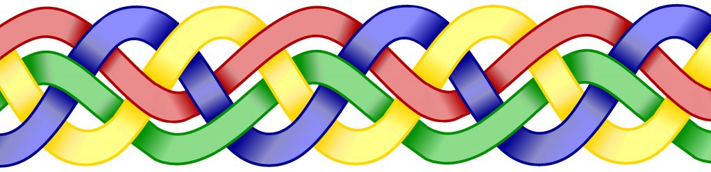
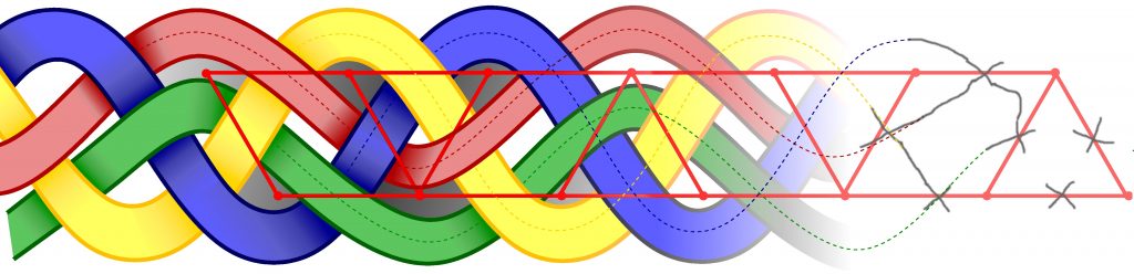
Friezes and tilings frequently accompany the teaching of isometries. The objects that we will consider in this vignette, like the one in Figure 1, are not far from them. However, their understanding involves other mathematics: topology and the theory of graphs, which are more recent than geometry. They constitute a fabulous subject to makes you feel and experience the power of mathematics, its delicacy and rigor.
Figure 1. A braid with four ribbons forming a frieze.
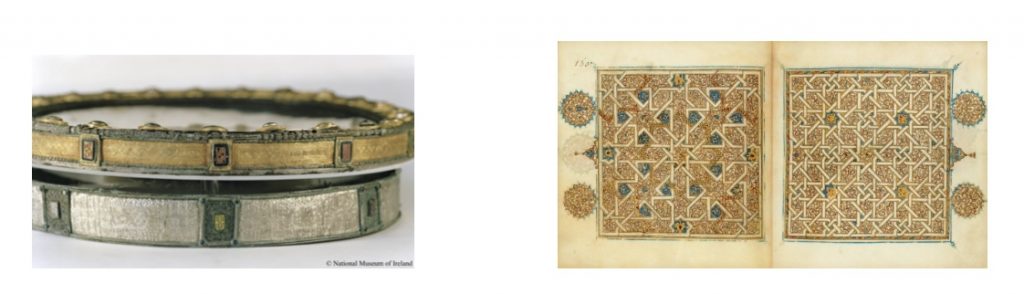
Knots and links have been used in many civilizations as tools and ornaments, from Celtic epic sculptures to Persian illuminations of the Koran (Figure 2).›
They appear in the lives of fishermen and basket makers, and when we lace our shoes or braid our hair. They are extremely diverse and mathematics can help to order this diversity, by questioning what brings together or differentiates these shapes. This study is part of topology and in particular the branch of topology called knot theory.
Knot Theory
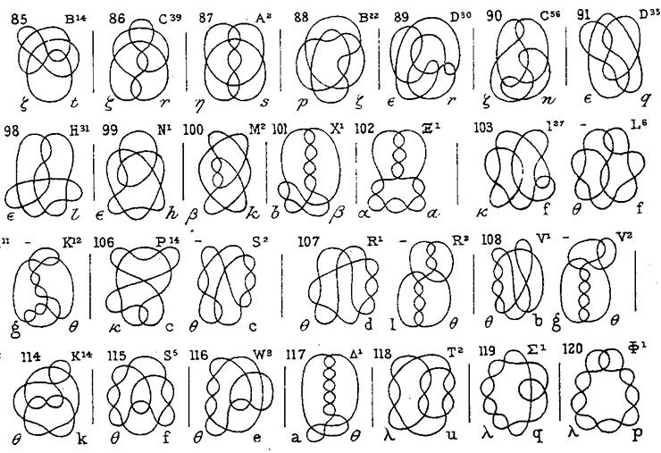
A knot is defined mathematically as an embedding of the circle in space. Practically, imagine a piece of string that we twist without cutting it, and retie the two ends. A link, on the other hand, is an assembly of several knots, several pieces of string. The illustration at the beginning of this vignette, for example, interlaces blue, red, yellow and green ribbons that pass over and under each other alternatively; it’s a braid. The theory of knots began to develop in the second half of the 19th century and its source is not strictly speaking mathematical. Physicists William THOMSON, better known as Lord KELVIN, and Peter Guthrie TAIT were among the first to contribute. They thought it would help them understand the phenomena of absorption and emission of light by atoms. And it lead TAIT to undertake a classification of knots (Figure 3).
FIGURE 3. Extracts from TAIT’s classification
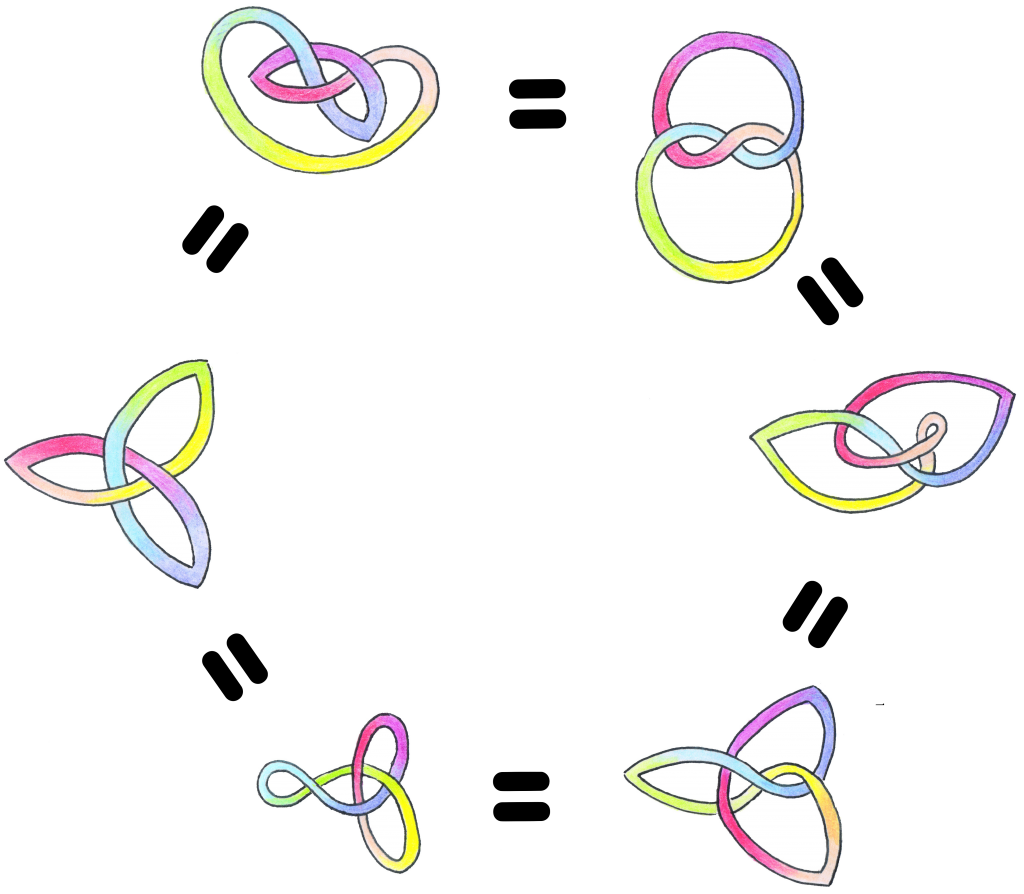
FIGURE 4. Trefoil
It is difficult to recognize that two knots are in the same class, i.e. that one can pass from one to the other by a continuous deformation, like when trying to untangle a string tied at its ends, without unraveling or cutting it. See for example these different images of the same trefoil knot (Figure 4), which is the simplest knot that is not trivial (i.e. which cannot be reduced to a circle).
This is why knot theory seeks to associate knots with quantities that these continuous deformations do not modify: invariants. For example, the polynomial of ALEXANDER is an invariant which associates a polynomial with integer coefficients to each type of knot. It was discovered by James Wadell ALEXANDER in 1923 and is the first invariant of this type. The ALEXANDER’s polynomial of the trefoil knot, for example, is: $t^2-t+1$. But first let’s learn how to draw a link. We will then come back to this question of invariants.
Links, Knots, and Graphs
A link (or a braid if it is open) is a knot with several components. It is generally represented by its regular projection in a plane: Its threads are drawn crossing transversely and at most two by two: there are not three points of the knot which are projected on the same point of the plane, the strands at the crossings have different projected directions, and the crosses are finite in number. To describe the object that results from these different crossings and its structure is not obvious.
This abstract model neglects a certain number of parameters such as the color of the strands and their thickness. It is a planar graph: with vertices connected by edges, not necessarily rectilinear, which do not intersect and we will label them with a left / right chirality.
Figure 5. Coloring
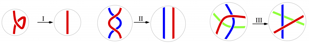
A regular projection of a link partitions the plane in different zones, delimited by the projection of the link itself. Where there are crossings, four zones meet locally. We can, according to JORDAN’s theorem,1 color all areas in two colors, say black and white, such that these crosses resemble a chessboard (two opposite zones have the same color and two contiguous zones have a different color).
It suffices to decide that the infinite exterior zone is white, to choose a point inside and connect each zone by a path which crosses transversely the projection of the interlacing and avoids crossings (Figure 5).
Each time you go through a thread, you change color. We show that the result does not depend on the chosen starting point, nor on the detail of the path followed and that we always end up with a consistent coloring. The coloring indeed depends only on the parity of the number of strands crossed. We associate a vertex with each black zone and we connect them by an edge, drawn above each crossing, from a black area to its opposite. We then attach the corresponding label to encode whether it is the right strand or the left strand which, seen from a vertex, passes above. The coding is consistent: the opposite zone gives the same chirality (Figure 6).
Figure 6. A left edge.
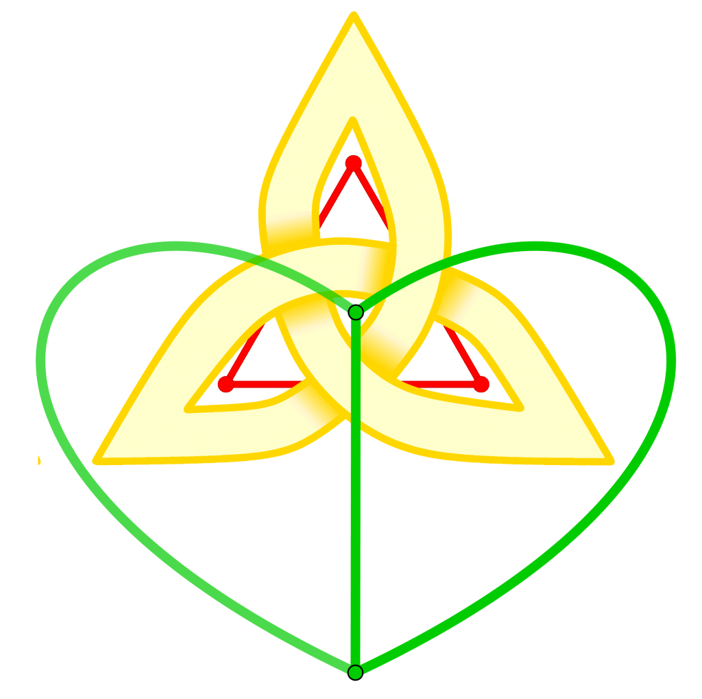
Figure 7. Two dual graphs of the trefoil knot.
The trefoil knot is thus associated with a triangle where all edges have the same chirality, say left: it is an alternating link: when you follow a strand, it crosses alternately above, below, above … But this is not the only graph which codes this knot, there is also a graph with two vertices and three edges. They are not straight but curved and labeled right! (Figure 7).
These two graphs are what are called dual graphs. This coding by a planar graph allows the interlacing to be completely coded and it is much easier to describe. The complicated braid is in fact encoded by a graph that can be explained in one sentence, for example, “a triangular ladder from which a rung is removed every three” (Figure 8).
FIGURE 8. A triangular ladder missing one rung every three encodes the braid.
These graphs are evocative and Alexander GROTHENDIECK called a large class of (locally) planar graphs children’s drawings . After this phase of analysis, let’s proceed to the synthesis: draw the interlacing encoded by a graph. This is done in three steps shown from right to left in Figure 8:
Draw a cross in the middle of each edge. Any cross is in the middle of an edge.
Connect the strands to each other in a continuous path.
Decide the above/below.
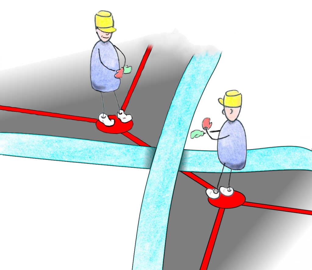
In detail, a cross is drawn in pencil, inclined between 30 and 60° with the edge. This orientation is important for the next stage because we continue each small strand along the ridge in the direction where it points. We thus arrive at the next crossing and we connect to the strand that points in that direction. At this stage, we do not introduce any new crossing and the strands do not cross the edges except at crossings. A useful metaphor: imagine the edges like the walls of a labyrinth, which we follow and which we cannot cross, except at crossroads, where a door appears (Figure 9).
Figure 9. The metaphor of the labyrinth: edges are walls, the crossings are doors.
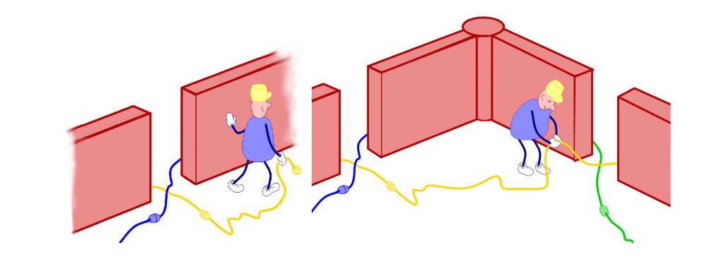
Finally, choosing a crossing, by aligning the edge that carries it with one’s gaze, identify which of the two strands comes from the right and which comes from the left. It allows you to replace the crossing by a “bridge” with a strand (say the left) passing above and the other (the right) below. We invite you now, before reading the rest, to draw up a small graph, of 5 or 6 edges, all of comparable lengths, angles not too sharp not too obtuse, and to develop the knot that it encodes. It suffices for this to play with planar graphs. The video http://video.math.cnrs.fr/entrelacs/ and the examples in [4, 5] can give you ideas.
3. Invariants
The first to take a serious interest in invariants was the young Carl Friedrich GAUSS at the beginning of the 19th century, describing the interlacing of two curves, $ \gamma_1, \gamma_2 $, in space, calculated as an impressive though integer valued integral,
This number is not calculated here from the projection of the interlacing but remains the same when we deform the curves without intersecting. It seems understandable if we are convinced that the result is an integer: the formula depends continuously on each curve and can only jump one unit when there is a problem: when the denominator vanishes, that is, when both curves intersect. But we can calculate it much more easily using a projection, by orienting the strands and simply summing signs for each crossing between the two curves: +1 for and -1 for . When there is only one curve, this combinatorial sum defines a number, that we call the writhe $w(K)$ of the projection of the node $K$. The right trefoil knot thus has a +3 writhe. But what becomes of $w(K)$ when incidents alter the projection? There are three types of complications which can occur in the projection of a knot. Let’s look locally in a small disc, the rest of the interlacing remaining the same as in Figure 10:
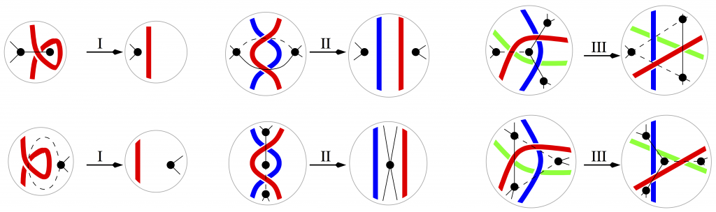
Figure 10: The three Reidemeister moves
In the twenties, BRIGGS and REIDEMEISTER demonstrated that the only simplifications we needed to go from one particular projection to any other were described by these three movements. To have a knot invariant is therefore to have a function whose value is not modified by these moves. But we quickly see that, whatever the strand orientations, if transformations II and III do not modify the writhe, the first one modifies it! The number $w(K)$ is therefore not a knot invariant!
However we can fix these problems and get real invariants. They are not simple numbers, but a collection of numbers, coefficients of polynomials in one or two variables.
The heroes of this part of the story are James Waddell ALEXANDER in 1923, John Horton CONWAY in 1969, Vaughan JONES in 1984 and Louis KAUFFMAN in 1987. They discovered, and others after them, by means touching algebra or mathematical physics, ways of building complex links functions as combinations of the same function but on simpler links: these are the skein relations. Among these functions, some are invariants. There are different versions on the same theme. In the same way as for the movements of REIDEMEISTER, we modify locally a link inside a small ball, leaving the rest unchanged.
KAUFFMAN’s bracket is defined by
its value $ = 1$ on the trivial knot,
its value with an extra unknot
$ = (- a^2-a^{- 2 }) $ and
the skein relation
$<$$> = a <$$> + a^{-1} <$$>$.
It suffers from the same problem as the writhe: the trivial knot’s bracket with writhe $-1$ is
$<$
$>=a<$
$> + a ^ {- 1} <$
$>
= a + a ^ { -1} (- a ^ 2-a ^ {- 2}) = a-a-a ^ {- 3} = -a ^ {- 3} \not = 1 $!
And every time we writhe, we multiply the result by that factor. Therefore, when we multiply by $ (- a) ^ {3w (K)} $, we get a true invariant! In the box below we calculate the KAUFMANN’s bracket of the standard trefoil knot of writhe $-3$. The crossings that are to be split are indicated by yellow discs.
$<$
$> = a<$
$> + a ^ {- 1}<$
$>$
where the first knot is the trivial twist knot of writhe 2 while the last is a link with two simple knotted components which is called the HOPF link.
It satisfies
$<$
$>=<$
$>$
$=a<$
$>+a^{-1}<$
$>$
$=a<$
$>+a^{-1}<$
$>$
$=a(-a^3)+a^{-1}(-a^{-3})=-a^4-a^{-4}$
that we replace above to yield
$<$
$> = a (- a ^ 3) ^ 2 + a ^ {- 1} (- a ^ 4-a ^ {- 4}) = a ^ 7-a ^ 3-a ^ {- 5} $.
We could also have applied three times the skein relations without thinking to obtain $ 2 ^ 3 = 8 $ terms. As the left trefoil has a twist of $ -3 $, the associated invariant is therefore $ (- a) ^ 9 (a ^ 7-a ^ 3-a ^ {-5}) = – a ^ {16} + a ^ {12} + a ^ 4 $. We can show that it is always a LAURENT polynomial (we allow negative degrees) of degree a multiple of 4 and by the change of variable $t = a^{−4}$ we obtain the JONES polynomial of 1984.
REIDEMEISTER moves and skein movements are also expressed on the graphs which code them (Figure 11 drawing in solid left edges, and in dashed right edges).
Figure 11. REIDEMEISTER’s moves on the graph.
On the graph, the skein relations amount to erasing the edge or fusing the vertices, which can be noted by crossing out the edge, respectively across or along. To the skein relation
$<$
$> = a <$
$> + a^{-1} <$
$>$
corresponds
$<$
$>= a<$
$>+ a ^ {- 1}<$
$>$,
each type of wall bringing a factor $ a $ or $ a ^ {- 1} $. In applying the relation on all the edges we end up with a disjoint union of trivial knots. Thus, the computation of KAUFMANN’s bracket of the trefoil can also be written:
$<$
$>=a<$
$>+a^{-1}<$
$>$
and iterating, it yields
$ = a (<$
$> +<$
$> + <$
$>) + a ^ 3<$
$> + a ^ {- 1} (<$
$> + <$
$> + <$
$>) + a ^ {- 3} <$
$> = 3a + a ^ 3 + 3a ^ {- 1} + a ^ {- 3}
= 3a + (a ^ 3 + 3a ^ {- 1}) (- a ^ 2-a ^ {- 2}) + a ^ {-
3} (- a ^ 2-a ^ {- 2}) ^ 2 = 3a- (a ^ 5 + a + 3 ^ a + 3a ^ {-
3}) + a + 2a ^ {- 3} + a ^ {- 7} = -a ^ 5-a ^ {- 3} + a ^ {-
7}. $
It is actually the KAUFFMAN’s bracket of the mirror trefoil.
This sum on all the possible contributions of local configurations is called a partition function in statistical mechanics.
The HOMFLY-PT polynomial2 of a knot $K$ is a little more elaborate, it requires that we orient the knot and needs two variables; $ P (x, y) (K) $ is thus defined by: $ P (O) = 1 $ and the skein relation
$ x P ($
$) – y P ($
$) = P ($
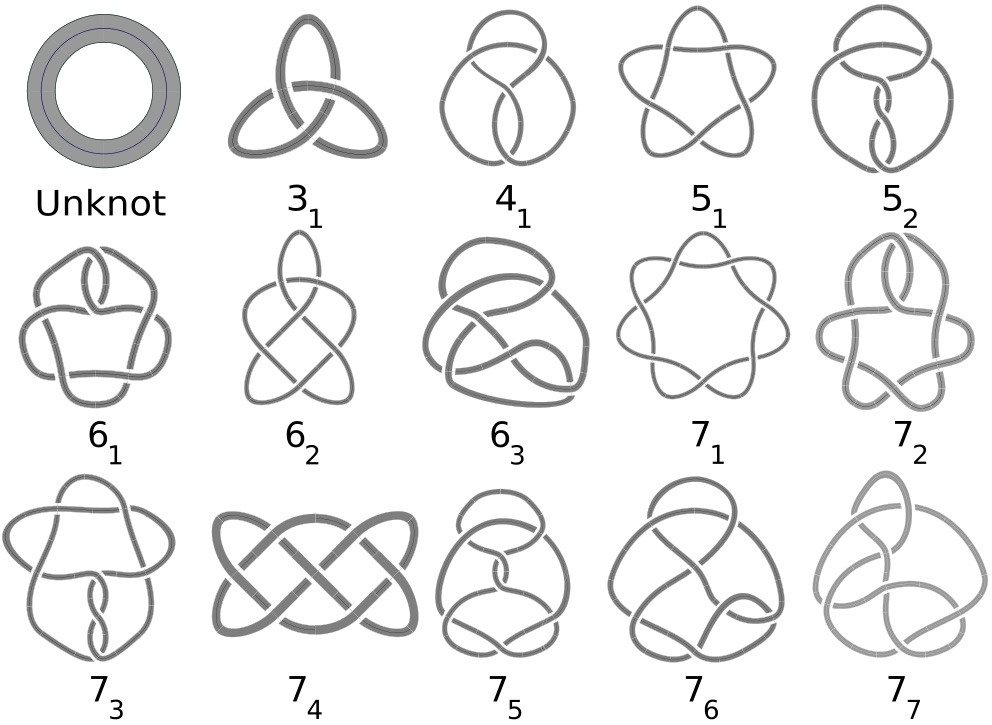
$)$. It has the big advantage of being compatible with the COMPOSITION of knots: the sum $ K_1 \sharp K_2 $ of two knots is obtained simply by opening them and gluing them back together. The polynomial of $ K_1 \sharp K_2 $ then satisfies $ P (x, y) (K_1 \sharp K_2) = P (x, y) (K_1) \times P (x, y) (K_2) $. Just as any integer can be decomposed as factors of prime numbers ($ 12 = 2 ^ 2 \times 3 $), knots can uniquely decompose into prime knots. It was the chemical intuition of KELVIN and TAIT. Figure lists the first prime knots with up to seven crossings;
FIGURE 12. The table of prime knots up to 7 crossings.
4. Conclusion
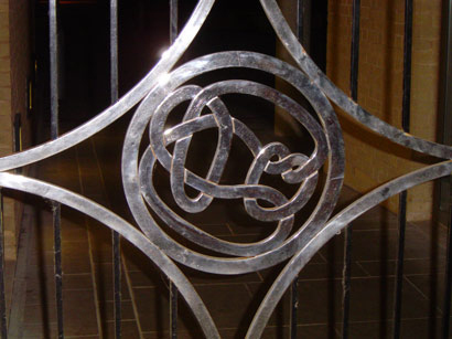
Interlacing first appeared in mankind as a technical tool, then as a manifestation of his artistic creativity, and then many centuries after, as objects of attention for scientists, physicists and mathematicians. The development of topology and its own tools made it possible to progress in the understanding of these objects, to identify invariants. However, many issues remain open and the research is very active there. Very recently, in 2020, for example, a conjecture concerning a fascinating knot (Figure 13) discovered by John CONWAY 50 years ago has been proved by the mathematician Lisa PICCIRILLO: she proves that this knot, which possesses the same ALEXANDER-CONWAY’s polynomial as the unknot, is not a slice knot [7].
FIGURE 13. The CONWAY knot on the door of the Cambridge Mathematics Department (CC By SA Atoll).
Certainly the initial hopes of THOMPSON and TAITS were betrayed because the assumptions on which they were based were proved to be wrong, but work on knots and braids has now various applications, in biology as one would expect, but also in robotics for example. Topology is not an object of secondary education and this is also not the case for graphs for many students, but the various experiments that were carried out on drawing knots in elementary school, proved to be very motivating and enriching for the students, allowing them to unexpectedly put mathematics to their service when gazing on the world and artistic creations. The entrelacs.net site bears witness to this. For the teacher’s perspective, gaining insight into the underlying mathematics is as well important and that’s the subject of this vignette.
JORDAN’s theorem expresses that any simple and closed curve of the plane delimits two connected components of the plane, one limited, the other not.
Standing for HOSTE, OCNEANU, MILLET, FREYD, LICKORISH, YETTER and PRZYTYCKI, TRACZYK.
References
A. Aubin. Nœuds sauvages imaginary.org.
L. H. Kauffman. Knots and Physics. 4th Ed, volume 53. Singapore: World Scientific, 4th ed. edition, 2013.
M. Launay. Une énigme de 50 ans résolue : Le nœud de Conway n’est pas bordant – micmaths.
C.Mercat.De beaux entrelacs, video AuDiMath, Images des Mathématiques. In A. Alvarez, editor, Destination Géométrie et Topologie Avec Thurston, Voyages En Mathématiques, pages 15–26. Le Pommier, 2013.
J.-P. Petit. Le Topologicon. Les Aventures d’Anselme Lanturlu. Belin, Savoir sans frontières edition, 1981.
L. Piccirillo. How you too can solve 50+ year old problems – talks at google.
D. Rolfsen. Knots and Links. 2nd Print. with Corr, volume7. Houston, TX: Publish or Perish, 2nd print. with corr. edition, 1990.
A. Sossinsky. Knots. Origins of a mathematical theory. Paris: Éditions du Seuil, 1999.
Renate Tobies is a renowned historian of mathematics and natural sciences. As a profound researcher, she has been studying Felix Klein and his works for decades. As a quintessence of these studies, she has now presented a book on Felix Klein that can be considered the most comprehensive and scientifically in-depth biography, which also offers new insights into his life and work. However, this book sheds light not only on Klein’s life and mathematical work, but also on his commitment to reforms in mathematics education and other fields.
Seen up close, a snowflake reveals all sorts of splendors: a marvel of geometry and symmetry. In 1610, the great astronomer Johannes Kepler was astonished and wanted to explain why snowflakes have six branches.
Etienne Ghys has in turn become fascinated by snowflakes. In this book with magnificent images, he tells us the story of the science of snow. Along the way, we meet some picturesque and learned characters, a Swedish archbishop, a French philosopher and an English scientist, others Dutch, American, Japanese, without forgetting “a Lady” and a whale fisherman.
Little by little, we learn that the shape of crystals is linked to the temperature and humidity of the place where they are formed. That by observing a flake, we can know the state of the atmosphere which overhangs us…
Etienne Ghys, with his unequalled talent for writing, makes us discover a whole science. The tone is warm, the story leads us. We reach the steps of the most modern science and we see, by very simple illustrations, the mathematical horizon of crystallography.A wonderful initiatory journey, for all ages. A book where poetry and science are mixed. A book for everyone.
by Giulia Signorini, Michele Tocchet, both from “Liceo Filippo Buonarroti” in Pisa, and Anna Baccaglini-Frank, University of Pisa.
In 1871 Felix Klein published two papers, called “On the so-called non-Euclidean geometry”, in which he proposed to call the first type of geometry “elliptic geometry” (from the Greek ellipsis, that means omission) and the second type “hyperbolic geometry” (form the Greek hyperbola, that means excessive). A good model for elliptic geometry is the sphere.
Circle inversion provides an interesting example of geometric transformation that, unlike the affinities and isometries studied in high school, usually does not transform lines into lines (but into circles) and that can be presented in an elementary way since its properties can be explored with dynamic geometry software and easily proved in synthetic geometry. Indeed, some high school textbooks introduce circle inversion as an interesting topic of Euclidean geometry that can also be explored through dynamic geometry software.
IMAGINARY offers a platform for open and interactive mathematics with a variety of content that can be used in schools, at home, in museums, at exhibitions or for events and media activities. The main contents of IMAGINARY are its interactive programs and its picture galleries. IMAGINARY was initiated at the Mathematisches Forschungsinstitut Oberwolfach (MFO), an institute of the Leibniz Association. The MFO is a shareholder of IMAGINARY.
The Global Math Project is a worldwide movement committed to inspiring educators everywhere to ignite and sustain in their students a love for learning mathematics. The ultimate goal of the Global Math Project is demonstrating, in a genuine and direct way, that classroom mathematics can and does, in and of itself, serve as a portal to a genuine, meaningful, and connected human experience. They want especially to prove that curriculum-relevant mathematics is uplifting for the mind and for the heart.
by Nitsa Movshovitz-Hadar (Technion – Israel Institute of Technology)
Did
you know? – Over 125,000 new items are added each year, to the
international database managed by the American Mathematical Society
called MathSciNet®1
A vast majority of these items contain new results, continuously
enriching the ever-growing discipline known as Mathematics2.
To celebrate these tremendous achievements, all to be credited to the
incredible creativity of mathematicians, several valuable awards have
been established. This vignette is about a few of the more
prestigious ones. It opens with the two that nowadays are often
described as the Nobel Prize in mathematics3:
the Fields Medal and the Abel Prize.
The Fields Medal
The Fields Medal is one of two awards often described as the Nobel Prize of mathematics. It consists of a gold medal bearing the profile of Archimedes and a cash amount of 15,000 Canadian dollars (or roughly \$11,540). It is awarded to 2-4 mathematicians every four years at the opening ceremony of the ICM – International Congress of Mathematicians, to recognize outstanding mathematical achievement for existing work and the promise of future achievement. A candidate’s 40th birthday must not occur before January 1st of the year of the Congress at which the Fields Medals are awarded. (Recall, Andrew Wiles, who proved the long-standing Fermat’s Conjecture, missed it as he was slightly over 40 when he and Taylor took care of the final polish of the proof.4)
The Mathematics News Snapshots for High School (MNS) project aims to provide high school students with a glimpse into the exciting and dynamic world of contemporary mathematics. The project was founded in order to decrease the gap between the ever-growing nature of mathematics and the stagnated nature of school curricula. In this sense the project is exactly in line with the Klein-Project.
The Snapshots are designed and written by teams of experts in mathematics and mathematics education, directed by Prof. Nitsa Movshovitz-Hadar (Technion – Israel Institute of Technology).
The International Day of Mathematics (IDM) is a worldwide celebration.
Each year on March 14 all countries will be invited to participate through activities for both students and the general public in schools, museums, libraries and other spaces.
The International Day of Mathematics is a project led by the International Mathematical Union with the support of numerous international and regional organizations.


